3) Stripped-down poker

In this tutorial, we’ll create an extensive-form representation of a one-card poker game from Reiley et al (2008), a classroom game under the name “stripped-down poker”. This is perhaps the simplest interesting game with imperfect information.

We’ll use “stripped-down poker” to demonstrate and explain the following with Gambit:

1. Setting up an extensive-form game with imperfect information using information sets

2. Computing and interpreting Nash equilibria and understanding mixed behaviour and mixed strategy profiles

3. Acceptance criteria for Nash equilibria

In our version of the game, there are two players, Alice and Bob, and a deck of cards, with equal numbers of King and Queen cards.

• The game begins with each player putting $1 in the pot.

  • A card is dealt at random to Alice.

  • Alice observes her card.

  • Bob does not observe the card.

• Alice then chooses either to Bet or to Fold.

  • If she chooses to Fold, Bob wins the pot and the game ends.

  • If she chooses to Bet, she adds another $1 to the pot.

• Bob then chooses either to Call or Fold.

  • If he chooses to Fold, Alice wins the pot and the game ends.

  • If he chooses to Call, he adds another $1 to the pot.

• There is then a showdown, in which Alice reveals her card.

  • If she has a King, then she wins the pot.

  • If she has a Queen, then Bob wins the pot.

In addition to pygambit, this tutorial introduces the gtdraw package, which can be used to draw extensive form games in Python. gtdraw is optional here; if it isn’t available, the drawing cells below print a short note. To install gtdraw, see gtdraw. Another option for visualising extensive form games is to install the Gambit GUI and use it to load a saved EFG file.

try:
    from gtdraw import draw
except ImportError:
    def draw(*args, **kwargs):
        print(
            "gtdraw is not installed, so the game tree cannot be drawn here; "
            "see https://www.gambit-project.org/gtdraw/ to install it."
        )

import pygambit as gbt

Create the game with two players:

g = gbt.Game.new_tree(
    players=["Alice", "Bob"],
    title="Stripped-Down Poker: a simple game of one-card poker from Reiley et al (2008)."
)

In addition to the two named players, Gambit also instantiates a chance player internally to represent moves of chance. It isn’t exposed as a value you can access directly – Game.players lists only the personal players; chance moves are identified via Node.event instead (see below).

list(g.players)

['Alice', 'Bob']

A move belonging to the chance player is called an event, and is created with append_event rather than append_move, since it requires the probability distribution over its actions to be specified explicitly. Like append_move, append_event takes an H-built selector identifying the node(s) to add the event at.

The first step in this game is that Alice is dealt a card which could be a King or Queen, each with probability 1/2.

To simulate this in Gambit, we create a chance event at the root node of the game, using gbt.H.path() to select it:

g.append_event(
    gbt.H.path(),
    actions={"King": gbt.Rational(1, 2), "Queen": gbt.Rational(1, 2)}
)

draw(g, color_scheme="gambit")

Information sets

In this game, information structure is important. Alice knows her card, so the two nodes at which she has the move are part of different information sets.

We’ll therefore need to append Alice’s move separately for each possible card, i.e. the scenarios where she has a King or a Queen. append_move takes an H-built selector describing which node(s) to add the move at; gbt.H.path(label) describes the node reached by taking the action labeled label from the root:

for card in ["King", "Queen"]:
    g.append_move(gbt.H.path(card), player="Alice", actions=["Bet", "Fold"])

draw(g, color_scheme="gambit")

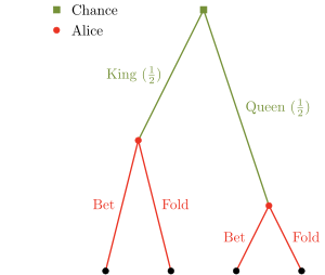
The loop above causes each of the newly-appended moves to be in new information sets, reflecting the fact that Alice’s decision depends on the knowledge of which card she holds.

In contrast, Bob does not know Alice’s card, and therefore cannot distinguish between the two nodes at which he has to make his decision:

• Chance player chooses King, then Alice Bets: gbt.H.path("King", "Bet")

• Chance player chooses Queen, then Alice Bets: gbt.H.path("Queen", "Bet")

In other words, Bob’s decision when Alice Bets with a Queen should be part of the same information set as Bob’s decision when Alice Bets with a King.

To set this scenario up in Gambit, we’ll need to add both possible moves as part of the same information set. This can be done with a single selector: gbt.H.path(..., "Bet") describes the node reached by any single action from the root (either card), followed by “Bet” – so it matches both of Bob’s decision nodes at once, joining them into one information set:

g.append_move(
    gbt.H.path(..., "Bet"),
    player="Bob",
    actions=["Call", "Fold"]
)

draw(g, color_scheme="gambit")

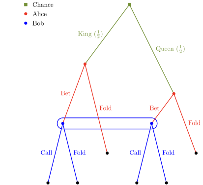
In game theory terms, this creates “imperfect information”. Bob cannot distinguish between these two nodes in the game tree, so he must use the same same probabilities for Call vs. Fold in both situations.

This is crucial in games where players must make decisions without full knowledge of the state of the game.

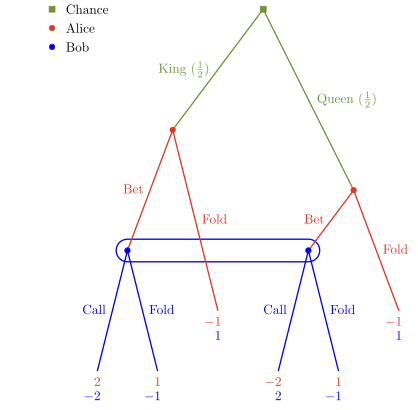
Let’s now set up the four possible payoff outcomes for the game, assigning each directly to the terminal node(s) it results at. We’ll label them according to player 1 (Alice):

# Alice folds, Bob wins small
g.make_outcome(
    gbt.H.path(..., "Fold"),
    {"Alice": -1, "Bob": 1},
    "Lose"
)

# Bob sees Alice Bet and calls, correctly believing she is bluffing, Bob wins big
g.make_outcome(
    gbt.H.path("Queen", "Bet", "Call"),
    {"Alice": -2, "Bob": 2},
    "Lose Big"
)

# Bob sees Alice Bet and calls, incorrectly believing she is bluffing, Alice wins big
g.make_outcome(
    gbt.H.path("King", "Bet", "Call"),
    {"Alice": 2, "Bob": -2},
    "Win Big"
)

# Bob does not call Alice's Bet, Alice wins small
g.make_outcome(
    gbt.H.path(..., "Bet", "Fold"),
    {"Alice": 1, "Bob": -1},
    "Win"
)

Outcome(game=Game(title='Stripped-Down Poker: a simple game of one-card poker from Reiley et al (2008).'), label='Win')

draw(g, color_scheme="gambit")

Computing and interpreting Nash equilibria

Since our one-card poker game has two players, we can use the lcp_solve algorithm in Gambit to compute a Nash equilibrium:

result = gbt.nash.lcp_solve(g)
result

NashComputationResult(method='lcp', rational=True, use_strategic=False, equilibria=[{'Alice': [{'Bet': Rational(1, 1), 'Fold': Rational(0, 1)}, {'Bet': Rational(1, 3), 'Fold': Rational(2, 3)}], 'Bob': [{'Call': Rational(2, 3), 'Fold': Rational(1, 3)}]}], parameters={'stop_after': None, 'max_depth': None})

The result of the calculation is returned as a NashComputationResult object.

The set of equilibria found is reported in NashComputationResult.equilibria; in this case, this is a list of MixedBehaviorProfile’s.

For one-card poker, we expect to find a single equilibrium (one MixedBehaviorProfile):

print("Number of equilibria found:", len(result.equilibria))
eqm = result.equilibria[0]

Number of equilibria found: 1

If we inspect the object type, we can see it’s a MixedBehaviorProfileRational which is a subclass of MixedBehaviorProfile that uses rational numbers for probabilities:

type(eqm)

pygambit.gambit.MixedBehaviorProfileRational

A mixed behavior profile specifies, for each information set, the probability distribution over actions at that information set.

Indexing a mixed behaviour profile by a player gives a MixedBehavior, which specifies probability distributions at each of the player’s information sets:

type(eqm["Alice"])

pygambit.gambit.MixedBehavior

eqm["Alice"]

$\left[\left\{\text{Bet}:1,\text{Fold}:0\right\},\left\{\text{Bet}:\frac{1}{3},\text{Fold}:\frac{2}{3}\right\}\right]$

In this case, at Alice’s first information set, the one at which she has the King, she always Bets.

At her second information set, where she has the Queen, she sometimes bluffs, raising with probability one-third.

The probability distribution at an information set is represented by a MixedAction.

A MixedBehavior is a collection of these, one per information set belonging to the player; iterating over it does exactly that:

for number, (_infoset, mixed_action) in enumerate(eqm["Alice"], start=1):
    print(
        f"At information set {number}, "
        f"Alice plays Bet with probability: {mixed_action['Bet']}"
        f" and Fold with probability: {mixed_action['Fold']}"
    )

At information set 1, Alice plays Bet with probability: 1 and Fold with probability: 0
At information set 2, Alice plays Bet with probability: 1/3 and Fold with probability: 2/3

We can alternatively iterate through each of a player’s actions like so:

Indexing the profile directly by a Node requires identifying it with a Selector, since MixedBehaviorProfile.__getitem__ accepts only a player label or a Selector, not a bare Node.

A Node’s own path of action labels back to the root builds exactly the Selector that matches it:

def selector_for_node(node):
    labels = []
    current = node
    while current.parent is not None:
        labels.append(current.prior_action.label)
        current = current.parent
    labels.reverse()
    return gbt.H.path(*labels)

for number, node in enumerate(g.get_infosets("Alice"), start=1):
    for action in node.actions:
        print(
            f"At information set {number}, "
            f"Alice plays {action} with probability: {eqm[selector_for_node(node)][action]}"
        )

At information set 1, Alice plays Bet with probability: 1
At information set 1, Alice plays Fold with probability: 0
At information set 2, Alice plays Bet with probability: 1/3
At information set 2, Alice plays Fold with probability: 2/3

Now let’s look at Bob’s strategy:

eqm["Bob"]

$\left[\left\{\text{Call}:\frac{2}{3},\text{Fold}:\frac{1}{3}\right\}\right]$

Bob Calls Alice’s Bet two-thirds of the time.

Since Bob has just one information set, we can get its representative node and index the profile directly by it to read off a single action’s probability:

(bob_node,) = g.get_infosets("Bob")
eqm[selector_for_node(bob_node)]["Call"]

$\frac{2}{3}$

Because this is an equilibrium, Bob is indifferent between the two actions at his information set, meaning he has no reason to prefer one action over the other, in expectation, given Alice’s expected strategy.

MixedBehaviorProfile.action_values returns the expected payoff of taking each action, conditional on reaching its information set, grouped by information set:

bob_action_values = eqm.action_values[bob_node]
for action in bob_node.actions:
    print(
        f"When Bob plays {action} his expected payoff is {bob_action_values[action]}"
    )

When Bob plays Call his expected payoff is -1
When Bob plays Fold his expected payoff is -1

Bob’s indifference between his actions arises because of his beliefs given Alice’s strategy.

MixedBehaviorProfile.beliefs returns the probability of reaching each node, conditional on its information set being reached.

Recall that the two nodes in Bob’s only information set are g.root.children["King"].children["Bet"] and g.root.children["Queen"].children["Bet"]):

for node in bob_node.members:
    print(
        f"Bob's belief in reaching the {node.parent.prior_action.label} -> "
        f"{node.prior_action.label} node is: {eqm.beliefs[node]}"
    )

Bob's belief in reaching the King -> Bet node is: 3/4
Bob's belief in reaching the Queen -> Bet node is: 1/4

Bob believes that, conditional on Alice raising, there’s a 3/4 chance that she has the King; therefore, the expected payoff to Calling is in fact -1 as computed.

MixedBehaviorProfile.infoset_probs returns the probability with which each information set is reached:

eqm.infoset_probs[bob_node]

$\frac{2}{3}$

The corresponding probability that a node is reached in the play of the game is given by MixedBehaviorProfile.realiz_probs, and the expected payoff to a player conditional on reaching a node is given by MixedBehaviorProfile.node_values:

bob_node_values = eqm.node_values["Bob"]
for node in bob_node.members:
    print(
        f"The probability that the node {node.parent.prior_action.label} -> "
        f"{node.prior_action.label} is reached is: {eqm.realiz_probs[node]}. ",
        f"Bob's expected payoff conditional on reaching this node is {bob_node_values[node]}"
    )

The probability that the node King -> Bet is reached is: 1/2.  Bob's expected payoff conditional on reaching this node is -5/3
The probability that the node Queen -> Bet is reached is: 1/6.  Bob's expected payoff conditional on reaching this node is 1

The overall expected payoff to a player given the behavior profile is returned by MixedBehaviorProfile.payoffs:

eqm.payoffs["Alice"]

$\frac{1}{3}$

eqm.payoffs["Bob"]

$\frac{-1}{3}$

The equilibrium computed expresses probabilities in rational numbers.

Because the numerical data of games in Gambit are represented exactly, methods which are specialized to two-player games, lp_solve, lcp_solve, and enummixed_solve, can report exact probabilities for equilibrium strategy profiles.

This is enabled by default for these methods.

When a game has an extensive representation, equilibrium finding methods default to computing on that representation. It is also possible to compute using the strategic representation. pygambit transparently computes the reduced strategic form representation of an extensive game:

g.get_strategies("Alice")

['1', '2', '3', '4']

In the strategic form of this game, Alice has four strategies.

The generated strategy labels list the action numbers taken at each information set. For example, label ‘11’ refers to the strategy gets dealt the King, then Bets.

We can therefore apply a method which operates on a strategic game to any game with an extensive representation.

gnm_result = gbt.nash.gnm_solve(g)
gnm_result

NashComputationResult(method='gnm', rational=False, use_strategic=True, equilibria=[{'Alice': {'1': 0.33333333333866677, '2': 0.6666666666613335, '3': 0.0, '4': 0.0}, 'Bob': {'1': 0.6666666666559997, '2': 0.3333333333440004}}], parameters={'perturbation': {'Alice': {'1': 1.0, '2': 0.0, '3': 0.0, '4': 0.0}, 'Bob': {'1': 1.0, '2': 0.0}}, 'end_lambda': -10.0, 'steps': 100, 'local_newton_interval': 3, 'local_newton_maxits': 10})

gnm_solve can be applied to any game with any number of players, and uses a path-following process in floating-point arithmetic, so it returns profiles with probabilities expressed as floating-point numbers.

This method operates on the strategic representation of the game, so the returned results are of type MixedStrategyProfile (specifically MixedStrategyProfileDouble):

gnm_eqm = gnm_result.equilibria[0]
type(gnm_eqm)

pygambit.gambit.MixedStrategyProfileDouble

Indexing a MixedStrategyProfile by a player gives the probability distribution over that player’s strategies only.

The expected payoff to each strategy is given by MixedStrategyProfile.strategy_values, grouped by player, and the overall expected payoff to each player is given by MixedStrategyProfile.payoffs:

gnm_payoffs = gnm_eqm.payoffs
gnm_strategy_values = gnm_eqm.strategy_values
for player in g.players:
    print(
        f"{player}'s expected payoffs playing:"
    )
    for strategy in g.get_strategies(player):
        print(
            f"Strategy {strategy}: {gnm_strategy_values[player][strategy]:.4f}"
        )
    print(
        f"{player}'s overall expected payoff: {gnm_payoffs[player]:.4f}"
    )
    print()

Alice's expected payoffs playing:
Strategy 1: 0.3333
Strategy 2: 0.3333
Strategy 3: -1.0000
Strategy 4: -1.0000
Alice's overall expected payoff: 0.3333

Bob's expected payoffs playing:
Strategy 1: -0.3333
Strategy 2: -0.3333
Bob's overall expected payoff: -0.3333

When a game has an extensive representation, we can convert freely between a mixed strategy profile and the corresponding mixed behaviour profile representation of the same strategies using MixedStrategyProfile.as_behavior and MixedBehaviorProfile.as_strategy.

• A mixed strategy profile maps each strategy in a game to the corresponding probability with which that strategy is played.

• A mixed behaviour profile maps each action at each information set in a game to the corresponding probability with which the action is played, conditional on that information set being reached.

Let’s convert the equilibrium we found using gnm_solve to a mixed behaviour profile and iterate through the players actions to show their expected payoffs, comparing as we go with the payoffs found by lcp_solve:

for player in g.players:
    print(
        f"{player}'s expected payoffs:"
    )
    gnm_action_values = gnm_eqm.as_behavior().action_values
    lcp_action_values = eqm.action_values
    for number, node in enumerate(g.get_infosets(player), start=1):
        for action in node.actions:
            print(
                f"At information set {number}, "
                f"when playing {action} - "
                f"gnm: {gnm_action_values[node][action]:.4f}"
                f", lcp: {str(lcp_action_values[node][action])}"
            )
    print()

Alice's expected payoffs:
At information set 1, when playing Bet - gnm: 1.6667, lcp: 5/3
At information set 1, when playing Fold - gnm: -1.0000, lcp: -1
At information set 2, when playing Bet - gnm: -1.0000, lcp: -1
At information set 2, when playing Fold - gnm: -1.0000, lcp: -1

Bob's expected payoffs:
At information set 1, when playing Call - gnm: -1.0000, lcp: -1
At information set 1, when playing Fold - gnm: -1.0000, lcp: -1

Acceptance criteria for Nash equilibria

Some methods for computing Nash equilibria operate using floating-point arithmetic and/or generate candidate equilibrium profiles using methods which involve some form of successive approximations. The outputs of these methods therefore are in general \(\varepsilon\)-equilibria, for some positive \(\varepsilon\).

\(\varepsilon\)-equilibria (from Wikipedia):

In game theory, an epsilon-equilibrium, or near-Nash equilibrium, is a strategy profile that approximately satisfies the condition of Nash equilibrium. In a Nash equilibrium, no player has an incentive to change his behavior. In an approximate Nash equilibrium, this requirement is weakened to allow the possibility that a player may have a small incentive to do something different.

Given a game and a real non-negative parameter \(\varepsilon\), a strategy profile is said to be an \(\varepsilon\)-equilibrium if it is not possible for any player to gain more than \(\varepsilon\) in expected payoff by unilaterally deviating from his strategy. Every Nash Equilibrium is an \(\varepsilon\)-equilibrium where \(\varepsilon = 0\).

To provide a uniform interface across methods, where relevant Gambit provides a parameter maxregret, which specifies the acceptance criterion for labeling the output of the algorithm as an equilibrium. This parameter is interpreted proportionally to the range of payoffs in the game. Any profile returned as an equilibrium is guaranteed to be an \(\varepsilon\)-equilibrium, for \(\varepsilon\) no more than maxregret times the difference of the game’s maximum and minimum payoffs.

As an example, consider solving our one-card poker game using logit_solve. The range of the payoffs in this game is 4 (from +2 to -2):

g.max_payoff, g.min_payoff

(Rational(2, 1), Rational(-2, 1))

logit_solve is a globally-convergent method, in that it computes a sequence of profiles which is guaranteed to have a subsequence that converges to a Nash equilibrium.

The default value of maxregret for this method is set at 1e-8:

logit_solve_result = gbt.nash.logit_solve(g, maxregret=1e-8)
len(logit_solve_result.equilibria)

1

ls_eqm = logit_solve_result.equilibria[0]
ls_eqm.max_regret()

2.6582744783176793e-08

The value of MixedBehaviorProfile.max_regret of the computed profile exceeds 1e-8 measured in terms of payoffs of the game. However, when considered relative to the scale of the game’s payoffs, we see it is less than 1e-8 of the payoff range, as requested:

ls_eqm.max_regret() / (g.max_payoff - g.min_payoff)

6.645686195794198e-09

In general, for globally-convergent methods especially, there is a tradeoff between precision and running time.

We could instead ask only for an \(\varepsilon\)-equilibrium with a (scaled) \(\varepsilon\) of no more than 1e-4:

(
    gbt.nash.logit_solve(g, maxregret=1e-4).equilibria[0]
    .max_regret() / (g.max_payoff - g.min_payoff)
)

6.265863445534259e-05

The tradeoff comes from some methods being slow to converge on some games, making it useful instead to get a more coarse approximation to an equilibrium (higher maxregret value) which is faster to calculate:

%%time
gbt.nash.logit_solve(g, maxregret=1e-4)

CPU times: user 8.01 ms, sys: 0 ns, total: 8.01 ms
Wall time: 8.01 ms

NashComputationResult(method='logit', rational=False, use_strategic=False, equilibria=[{'Alice': [{'Bet': 1.0, 'Fold': 0.0}, {'Bet': 0.3338351656285656, 'Fold': 0.666164834417892}], 'Bob': [{'Call': 0.6670407651644306, 'Fold': 0.3329592348608147}]}], parameters={'first_step': 0.03, 'max_accel': 1.1})

%%time
gbt.nash.logit_solve(g, maxregret=1e-8)

CPU times: user 15.4 ms, sys: 0 ns, total: 15.4 ms
Wall time: 15.3 ms

NashComputationResult(method='logit', rational=False, use_strategic=False, equilibria=[{'Alice': [{'Bet': 1.0, 'Fold': 0.0}, {'Bet': 0.33333338649882943, 'Fold': 0.6666666135011707}], 'Bob': [{'Call': 0.6666667065407631, 'Fold': 0.3333332934592369}]}], parameters={'first_step': 0.03, 'max_accel': 1.1})

The convention of expressing maxregret scaled by the game’s payoffs standardises the behavior of methods across games.

For example, consider solving the poker game instead using liap_solve().

(
    gbt.nash.liap_solve(g.mixed_strategy_profile(), maxregret=1e-1)
    .equilibria[0].max_regret() / (g.max_payoff - g.min_payoff)
)

0.03657804319443689

If, instead, we double all payoffs, the output of the method is unchanged:

for outcome in g.outcomes:
    outcome["Alice"] = outcome["Alice"] * 2
    outcome["Bob"] = outcome["Bob"] * 2

(
    gbt.nash.liap_solve(g.mixed_strategy_profile(), maxregret=1e-1)
    .equilibria[0].max_regret() / (g.max_payoff - g.min_payoff)
)

0.03657804319443689

Representation of numerical data of a game

Payoffs to players and probabilities of actions at events are specified as numbers. Gambit represents the numerical values in a game in exact precision, using either decimal or rational representations.

To illustrate, consider a trivial game which just has one move for the chance player:

small_game = gbt.Game.new_tree()
small_game.append_event(gbt.H.path(), dict.fromkeys(["a", "b", "c"], gbt.Rational(1, 3)))
list(small_game.root.action_probs.values())

[Rational(1, 3), Rational(1, 3), Rational(1, 3)]

Here we specified an equal-probability distribution over the three actions, using pygambit’s Rational class, which is derived from Python’s fractions.Fraction, to represent the probabilities exactly.

Numerical data can be set as rational numbers. make_event forms a collection of nodes into an event with a given distribution; applied to a single node which is already an event, it resets the probabilities. Let’s use it to change the distribution, again with Rational numbers:

small_game.make_event(
    gbt.H.path(),
    {"a": gbt.Rational(1, 4), "b": gbt.Rational(1, 2), "c": gbt.Rational(1, 4)}
)
list(small_game.root.action_probs.values())

[Rational(1, 4), Rational(1, 2), Rational(1, 4)]

Numerical data can also be explicitly specified as decimal numbers:

small_game.make_event(
    gbt.H.path(),
    {"a": gbt.Decimal(".25"), "b": gbt.Decimal(".50"), "c": gbt.Decimal(".25")}
)
list(small_game.root.action_probs.values())

[Decimal('0.25'), Decimal('0.50'), Decimal('0.25')]

Although the two representations above are mathematically equivalent, pygambit remembers the format in which the values were specified.

Expressing rational or decimal numbers as above is verbose and tedious. pygambit offers a more concise way to express numerical data in games: when setting numerical game data, pygambit will attempt to convert text strings to their rational or decimal representation. The above can therefore be written more compactly using string representations:

small_game.make_event(gbt.H.path(), {"a": "1/4", "b": "1/2", "c": "1/4"})
list(small_game.root.action_probs.values())

[Rational(1, 4), Rational(1, 2), Rational(1, 4)]

small_game.make_event(gbt.H.path(), {"a": ".25", "b": ".50", "c": ".25"})
list(small_game.root.action_probs.values())

[Decimal('0.25'), Decimal('0.50'), Decimal('0.25')]

As a further convenience, pygambit will accept Python int and float values. int values are always interpreted as Rational values.

pygambit attempts to render float values in an appropriate Decimal equivalent. In the majority of cases, this creates no problems. For example:

small_game.make_event(gbt.H.path(), {"a": .25, "b": .50, "c": .25})
list(small_game.root.action_probs.values())

[Decimal('0.25'), Decimal('0.5'), Decimal('0.25')]

However, rounding can cause difficulties when attempting to use float values to represent values which do not have an exact decimal representation:

try:
    small_game.make_event(gbt.H.path(), {"a": 1/3, "b": 1/3, "c": 1/3})
except ValueError as e:
    print("ValueError:", e)

ValueError: Probabilities must sum to exactly one

This behavior can be slightly surprising, especially in light of the fact that in Python:

1/3 + 1/3 + 1/3

1.0

In checking whether these probabilities sum to one, pygambit first converts each of the probabilities to a Decimal representation, via the following method:

gbt.Decimal(str(1/3))

Decimal('0.3333333333333333')

…and the sum-to-one check then fails because:

gbt.Decimal(str(1/3)) + gbt.Decimal(str(1/3)) + gbt.Decimal(str(1/3))

Decimal('0.9999999999999999')

Setting payoffs for players also follows the same rules. Representing probabilities and payoffs exactly is essential, because pygambit offers (in particular for two-player games) the possibility of computation of equilibria exactly, because the Nash equilibria of any two-player game with rational payoffs and chance probabilities can be expressed exactly in terms of rational numbers.

It is therefore advisable always to specify the numerical data of games either in terms of Decimal or Rational values, or their string equivalents. It is safe to use int values, but float values should be used with some care to ensure the values are recorded as intended.

References

Reiley, David H., Michael B. Urbancic and Mark Walker. (2008) “Stripped-down poker: A classroom game with signaling and bluffing.” The Journal of Economic Education 39(4): 323-341.